The Portfolio Optimizer for Wealth Management

Direct Indexing can increase returns in taxable accounts

Summary

With Direct Indexing (DI), instead of buying a fund that tracks a stock index, we buy the individual stocks. DI can increase after-tax returns through tax loss harvesting.

Our backtests show an annualized improvement of 0.97% pre-tax and 0.56% after-tax. These are conservative, because the backtest period was a bull market, when DI has the fewest opportunities for loss harvesting.

Our DI implementation was written by the software developer who also wrote the code for the first mass-market, fully automated DI for a leading robo-advisor.

Background

The following assumes DI on a large-cap US equities stock index for a $1,000,000 account. The two largest constituents are AAPL at 4% and MSFT at 3% [Note: these are based on prices at a single point in time, because stock indexes are published in terms of shares, not dollar percentages, which change over time].

On day 1, we just buy each index constituent: $40,000 of AAPL, $30,000 of MSFT, etc. [Note: this gets more complicated in the presence of held-away assets.]

On subsequent days:

1. We generate tax loss harvesting sell orders: for each stock holding, we look at the lossy portion. If the average tax loss of the lossy tax lots exceeds a threshold (e.g. 1%), then we sell them. DI optionally creates a 'collar' of valid percentages of the total. Example: MSFT can be restricted to be within 1% of its 3% target, i.e. between 2% and 4%. Therefore, if MSFT is at 3.2% of the portfolio, and half of that is at a loss, we will only sell down to 2%, not to 1.6%.
2. Buy other stocks in the index, using the cash generated from the sells (or any other available cash from dividends, deposits, etc.) DI is different than plain TLH, because there is no notion of equivalent securities to replace the ones we sold: unlike ETFs where one can often find two that are very similar (e.g. with large cap equities), individual stocks will always be different enough to due idiosyncratic risk. However, even if that dissimilarity were acceptable, grouping index constituent stocks this way would be a tedious, manual, and subjective task. Instead, there are two main ways this can be done:
   • Pro rata: Target all buyable stocks to be equally misallocated, without regard to stock similarity.
   • Use a risk model to make the portfolio "look like" the index as much as possible, given the constraints. A risk model tells us in quantitative terms how similar one stock is to another. For example, if we sell Exxon Mobil, utilizing a risk model would push us towards buying Chevron.
   In step #2, we allow rebalancing (instead of buying only), because we may end up over-/underweight stocks for other reasons.

Scenario parameters

• Held by us: An initial $1,000,000 in cash, which we are free to invest.
• Deposits: $10,000 every month.
• Target allocation: 0.5% cash, 99.5% in a stock index. This is the case both when DI is enabled (where we hold the 311 stocks) and when it is disabled (where we buy a tracking ETF, which we construct for this backtest).
• Index details: to avoid licensing issues, we created a US large-cap 311-stock index. There are no index reconstitutions (additions, deletions, weight changes, etc.) to keep things simple.
• AUM fees: no fees, for simplicity. However, we support customized fee schedules; e.g. 25 bps annually, charged ~2 bps / month.
• Tax: both scenarios are for taxable accounts.
• Shares rounding: we only use round shares here, although we can support fractional shares and arbitrary rounding and order minimum amounts.
• Risk model: we have built our own risk model, and our DI can use it. However, we are not using it in this example, to keep things simple.

Results

Returns

We calculate portfolio totals using three sets of liquidation assumptions, which are labeled in the charts as follows:

1. Held by us: unrealized tax never has to be paid (e.g. charitable contributions, or step-up basis upon inheritance)
2. Held by us (liq. tax): the tax that would be owed at any given point in time gets if the portfolio were liquidated is subtracted from the portfolio value.
3. Held by us (liq. tax; ST taxed LT): long-term tax rates are applied even to short-term gains / losses. This metric is less realistic; however, we prefer it, because it avoids abrupt value changes around the days when short-term tax lots become long-term, such as one year after a large investment.

The fairest way to compare the results with vs. without DI is to look at the after-tax liquidation values. TLH strategies work by realizing losses today at the expense of postponing tax payments for later. Therefore, ignoring the fact that tax would have to be paid at some point would overstate the tax benefit of DI. However, pre-tax values can be useful as well. We can look at both; our software generates charts automatically, by running backtests over a multi-year period. Click on the following screenshots for an interactive version.

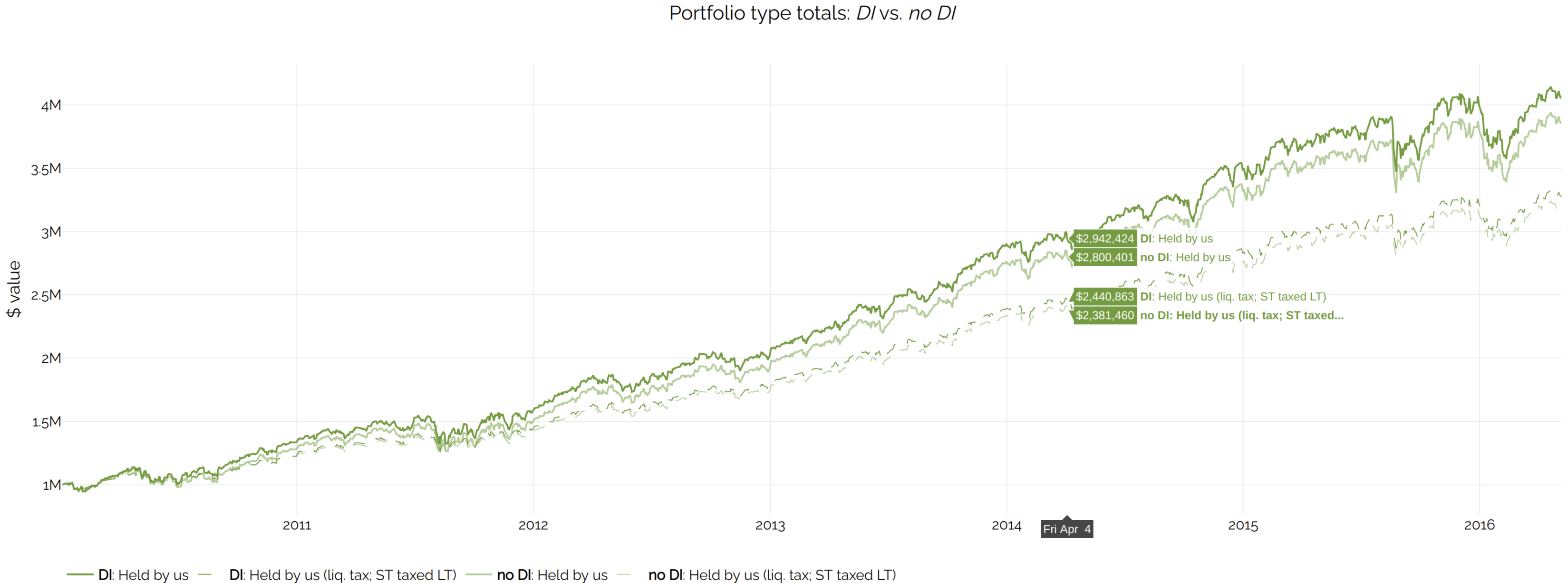
This shows portfolio values:

Note how the darker lines (DI) are higher than the lighter ones (no DI), regardless of liquidation assumptions. This means that DI (in this particular scenario, at least) increases returns. In the more realistic case where tax is eventually due - labeled Held by us (liq. tax; ST taxed LT) - the lines are closer together, as expected.

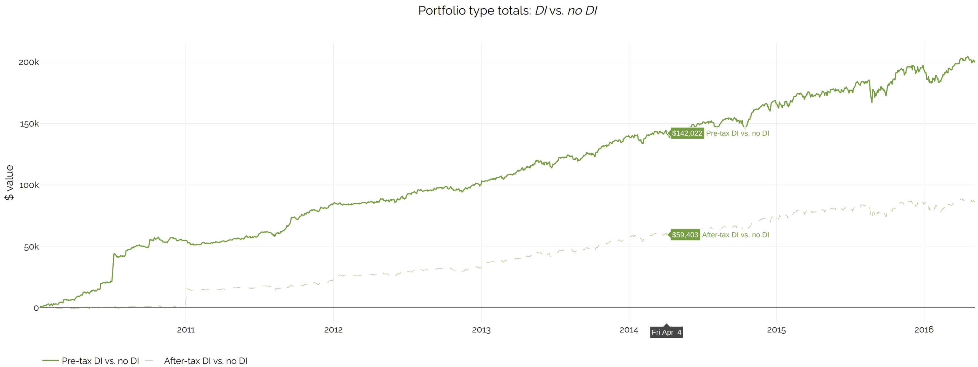
The improvement in pre-tax returns is the difference between the pair of solid lines above. Likewise for after-tax and the dashed lines. Those differences are easier to see when plotted separately:

These charts show that even the after-tax portfolio returns are higher with DI, not just the pre-tax returns. Note that the backtest period was mostly an up market; the benefit would have been considerably higher otherwise.

We can quantify the improvement. If we look for money-weighted returns in the data grids (the Summary button on the top left) for DI disabled vs. enabled, we can see the annualized difference is about 97 bps (1605.8 - 1509.2 bps) for pre-tax and 56 bps (1214.2 - 1157.9 bps) for after-tax returns, in this particular example.

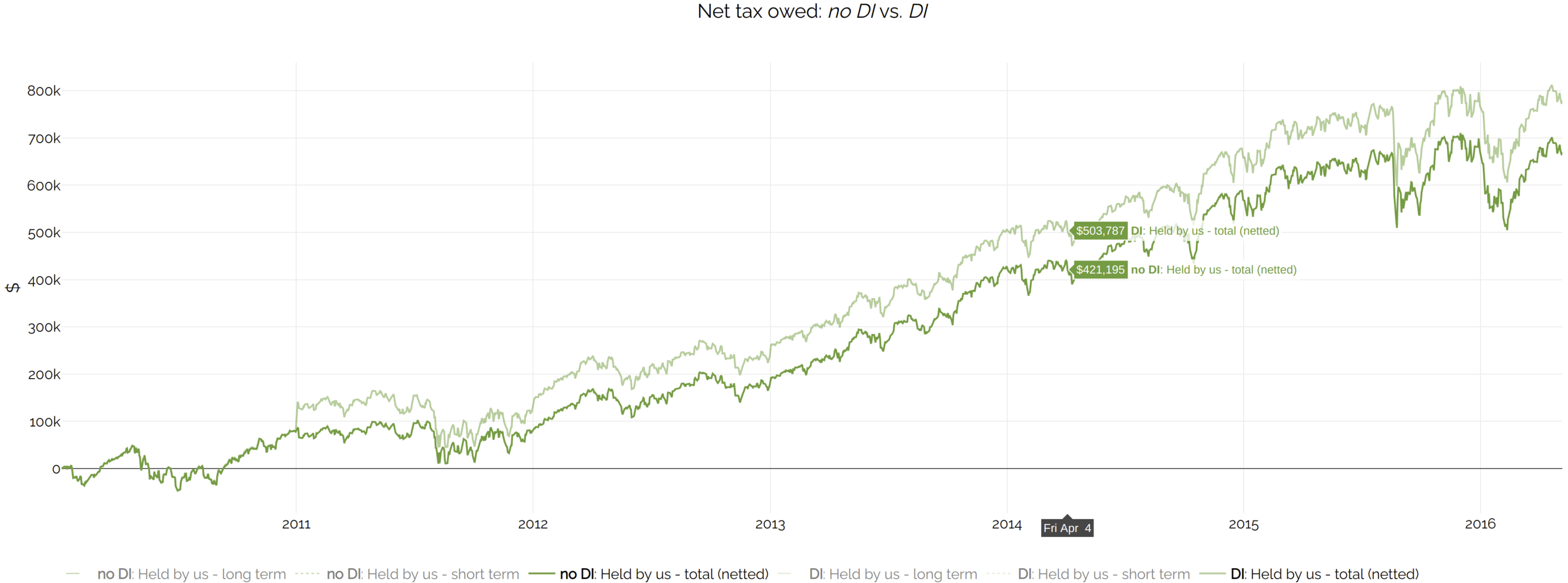
Net Tax Owed

It is also interesting to compare Net tax owed:

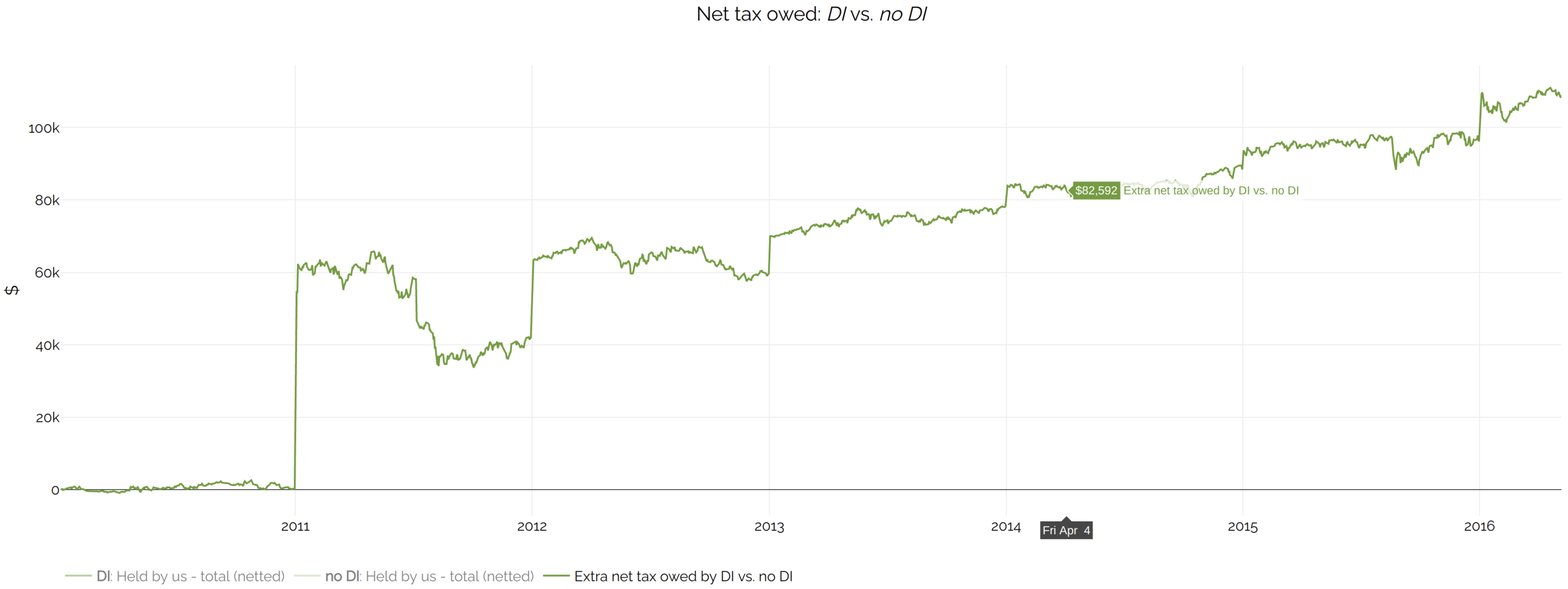
You can view the difference more clearly here:

.

DI results in more embedded gains over time. The charts indicate that DI has paid less in taxes, since more taxes have been deferred. Of course, all else being equal, it is better to owe less tax than more. However, in this case, more tax owed is a worthwhile price to pay, because the increased portfolio returns more than make up for it.

Tracking error

We can search for daily tracking error (standard deviation of period return diff), weighted by portfolio value, in bps in the data grids for DI. To convert to annualized numbers, we can multiply by 16 (approximate square root of number of trading days in a year).

With DI disabled, we buy an ETF that tracks the stock index perfectly, so the tiny tracking error we see (16 * 0.02 = 0.32 bps) is likely due to the cash drag from postponing the investment of any cash dividends, because we wait until there is enough cash in order to invest.

With DI enabled, annualized tracking error is 1.67 * 16 ~= 27 bps. This is a worthwhile price to pay given how much the returns improve. [Note: 27 bps is a measure of tracking variability, whereas the money-weighted returns improvement of 97 bps is a measure of performance. Therefore, the two are not directly comparable.]

Benefits of our technology

• Customization (investing): investing behavior is fully controllable at the API level; our DI currently has 30 tuning parameters, such as tax loss thresholds, tolerance bands for stock target percentages, how much to rely on the risk model (if at all), etc. Client-related settings such as marginal tax rates are also customizable, so that loss harvesting aggressiveness can decrease intelligently at lower tax brackets.
• Customization (presentation): we can show charts to end clients based on a their tax bracket and other inputs (deposit patterns, fees charged, external holdings, etc.), which helps with signing up new clients.
• DI on arbitrary indexes: those same charts also help investment research ascertain how well DI works for a new index, and to search for the best parameters (e.g. tolerance bands for stock targets). What would normally take days can now be done in minutes.
• Granular wash sale logic: we prevent wash sales at an individual tax lot level, not with blanket "do-not-sell" restrictions for a single stock, like many leading DI implementations do. This means that, if only a few tax lots would cause a wash sale if sold, we can still sell other lots. This makes a meaningful difference in practice.
• Testing: backtests are realistic, because the use the exact same Java code that would be used in production. This sounds obvious but it is not easy to do. This means that if any problems will be spotted during product development time, not on a live account at production time.
• Maximally realistic handling of taxes: The benefit of harvesting a tax loss is not assumed to accrue on the same day of the harvest. That would be expedient, but less accurate. Instead, we "do your taxes" on April 15th of every backtest year, and properly net short/long-term gains and losses to come up with the correct tax payment or refund. This is just one example of our meticulous attention to detail.
• Speed: using several sophisticated techniques, a single DI optimization takes less than 1 second. A multi-year DI backtest for our 311-stock index currently takes 5-10 minutes. Note that we have not even done any performance tuning yet, so there is plenty of scope for improvement.

Conclusion

DI can increase after-tax returns in managed accounts while incurring fairly modest tracking error.

Addendum

Why DI?

Advantages, in descending importance:

• Increase after-tax returns: similarly to simple ETF-pairs-based tax-loss harvesting (henceforth "plain TLH"), selling losses and keeping gains will usually increase after-tax returns, even when tax is paid eventually. This is mostly due to the time value of money, since the client stay invested in the market while postponing tax payments.
• Socially Responsible Investing (SRI) DI can invest less (or not at all) in stocks deemed undesirable to a client, effectively creating a personalized index. Naturally, the more the personalized index differs from the original one, the bigger the tracking error will be. DI for the purpose of SRI is also applicable to tax-deferred and non-taxable accounts. We intentionally did not the focus on SRI in this document.
• Reducing holding costs: if the ETFs that track an index have a high expense ratio, holding the individual constituents will typically be cheaper. This is rarely a problem in practice, because "DI-friendly" stock indexes (see 'prerequisites' section below) typically have cheap-expense-ratio ETFs that track them. Also, there can be other holding costs, because a broker may charge more for many small positions, instead of one large one. This does not happen with end-clients, but may happen to firms that use the broker.

Why does DI increase after-tax returns?

Just like plain TLH, after-tax returns are (on average) higher, because it is almost always better to postpone tax payments for later:

• Time value of money: any postponed upfront tax payment will instead get to grow with the market.
• For investors who will be in a lower tax bracket when they sell their assets later in life, they will owe less tax. [Note: Currently, assuming the tax law does not change, this benefit would be biggest for short-term capital gains, which get taxed at ordinary income rates, which can drop a lot during retirement. However, for a scenario of selling assets in retirement, the tax bracket benefit effectively applies only to long-term capital gains, where the differential would be limited to a possible avoidance of the 3.8% Medicare surtax.]
• There are cases where no tax is owed at all, e.g. when assets are passed down to someone's heirs, or in a charitable contribution.

Prerequisites for the index constituents

• Liquid and with low spreads: the average spread, weighted by index target percentage, must not be much bigger than that of an ETF that tracks the index. This is the case for most large-cap US stock indexes, but not so for small-cap ones.
• Easy to trade: this depends on who uses DI. Let us take an emerging markets index as an example. A fully automated, "robo-style" DI implementation will need to send electronic orders to US exchanges, but an emerging markets index is unlikely to have liquid ADRs for all of its constituents, so that will not work. On the other hand, firms that have few (but high-value) client accounts may be OK with a more manual approach. Therefore, trading a combination of ADRs, GDRs, and "ordinary shares" (on non-US exchanges) could be acceptable. [Note: if some index constituents are illiquid, foreign, or otherwise hard to trade, they could be excluded from DI, which would only operate on the rest of the index, although at the cost of more tracking error.]

When does DI improve after-tax returns the most?

• Dispersion: TLH exploits the asymmetric return profile of losses vs. gains: losses can be realized, so as to offset other capital gains (typically from outside the account), whereas gains do not have to be realized. If stocks are too similar, then we will have either all losses, or all gains. [Note: this is too long to explain in detail here.]
• Index breadth: if an index only has a few stocks (e.g. 20 or fewer), it may be hard to avoid tracking error.
• Additional deposits: DI works best when there are several tax lots to choose from. Periodically investment of cash dividends helps somewhat, but current low dividend yields limit this effect.
• Down markets: during an up market, there will fewer losses, and therefore fewer opportunities to harvest losses.
• Lower future tax rates:The bigger the tax rate differential, the bigger the benefit.
• Momentum: DI does not explicitly bet on the direction of prices, or (more generally) on the momentum vs. mean reversion aspect of the market regime. However, selling losses instead of holding on to them will also result in higher returns in a momentum-driven market.